Recent posts

Glencoe Mountain Rescue stretcher build

Background

Part of my first degree concerned composites manufacture, and I worked in this field for a while before my science career. I still get stuck into the occasional composite materials project, so a couple of years ago I was approached by Glencoe Mountain Rescue with an interesting request. Their fleet of stretchers was originally designed by Hamish MacInnes to cope with the demanding mountain terrain, but with production halted indefinitely, an alternative solution was sought.

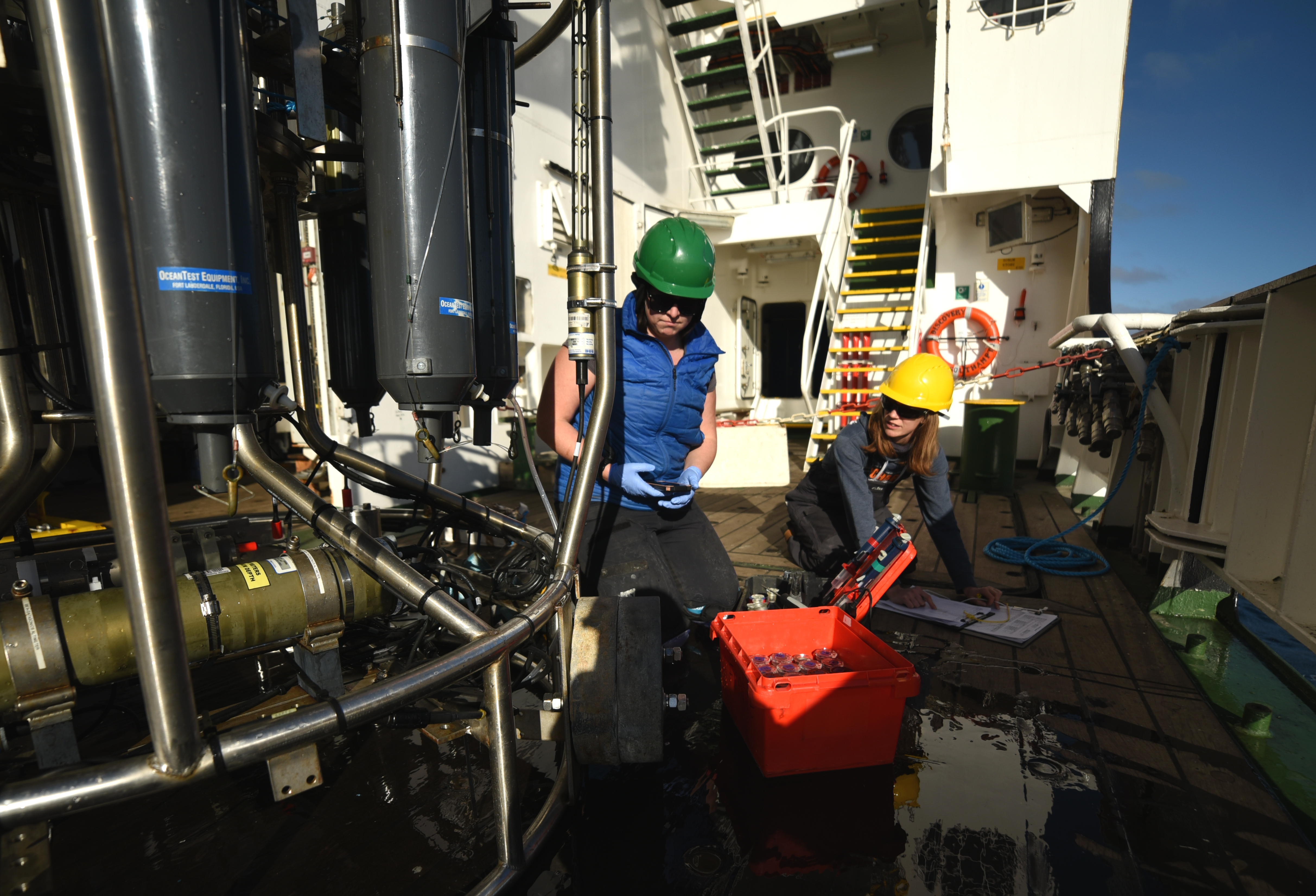
Many UK teams use titanium basket stretchers such as this linked example, but they are easily damaged by some of the more technical rescues, for example long cliff lowers, undertaken by the Glencoe team.

The challenge was therefore to build a strong, light skid tray which could be attached to an off-the-shelf stretcher to protect it from the rigours of rescues in rocky terrain. In particular, I aimed not only to build a working example for testing, but also to make a mould so that multiple stretchers could be similarly retrofitted with skid trays in the future. The stretcher is carried up the hill in two halves and is assembled for use, so the tray needed to be supplied in two closely fitting halves also.

Preparing the male ‘plug’ for moulding

The project was commenced by a GMR team member before other responsibilities got in the way, so the basic dimensions of the wooden ‘plug’, from which the mould would be formed, were already established. This saved time but it required a lot of modification to make it ready for moulding. The fibreglass mould will bond irrevocably to the plug if there is any surface roughness, porosity, or any mechanical locks preventing a clean release. The fight to separate a stuck mould from the plug usually damages or destroys both components.

One half of the wooden plug, from which the mould will be taken. The plug is shown sanded and filled, but needs additional preparation to make it ready for moulding.

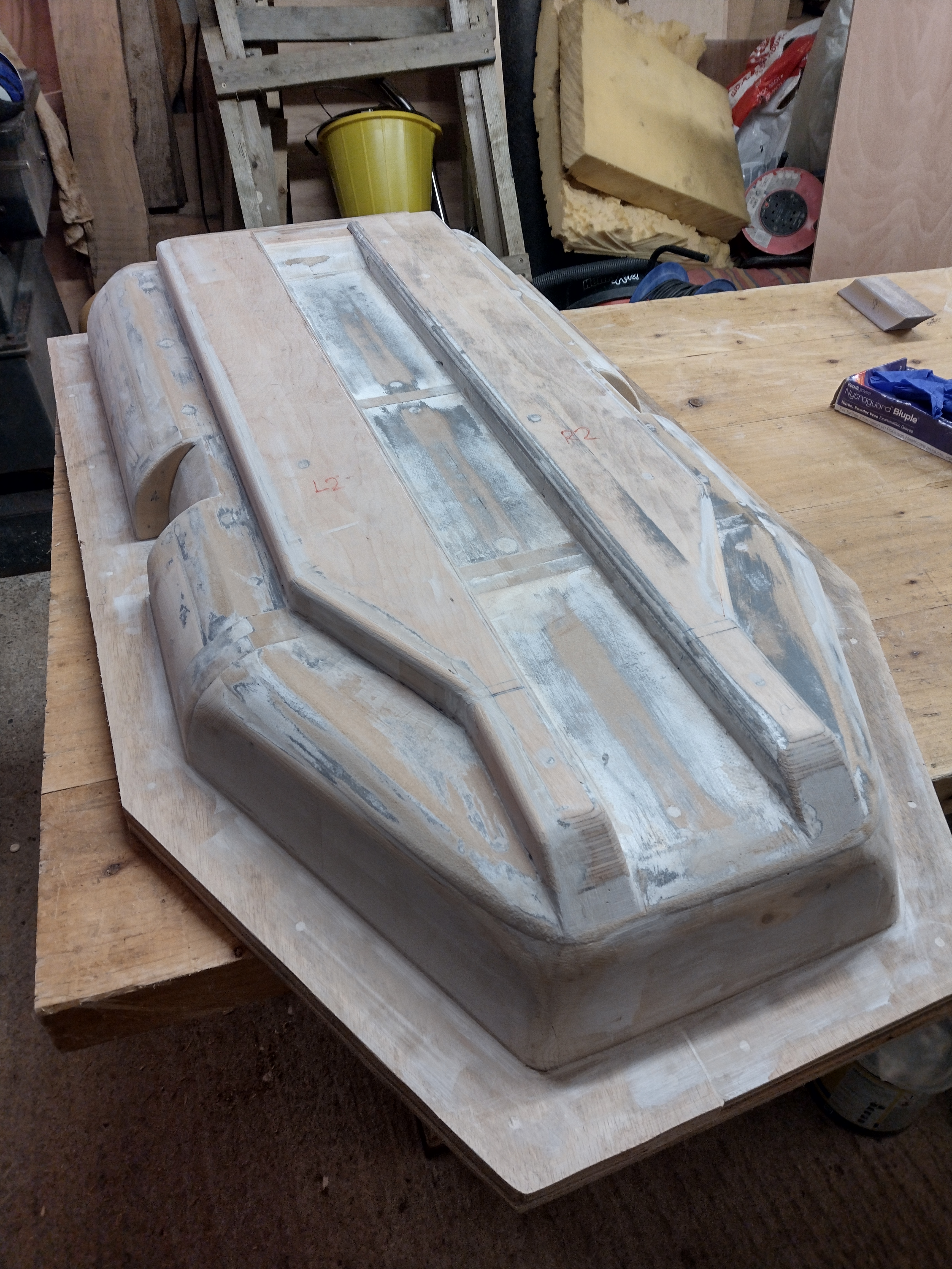
So began the long process of meticulously preparing the plug: elliminating imperfections with interminable rounds of sanding, filling and polishing until I could literally see my face in it.

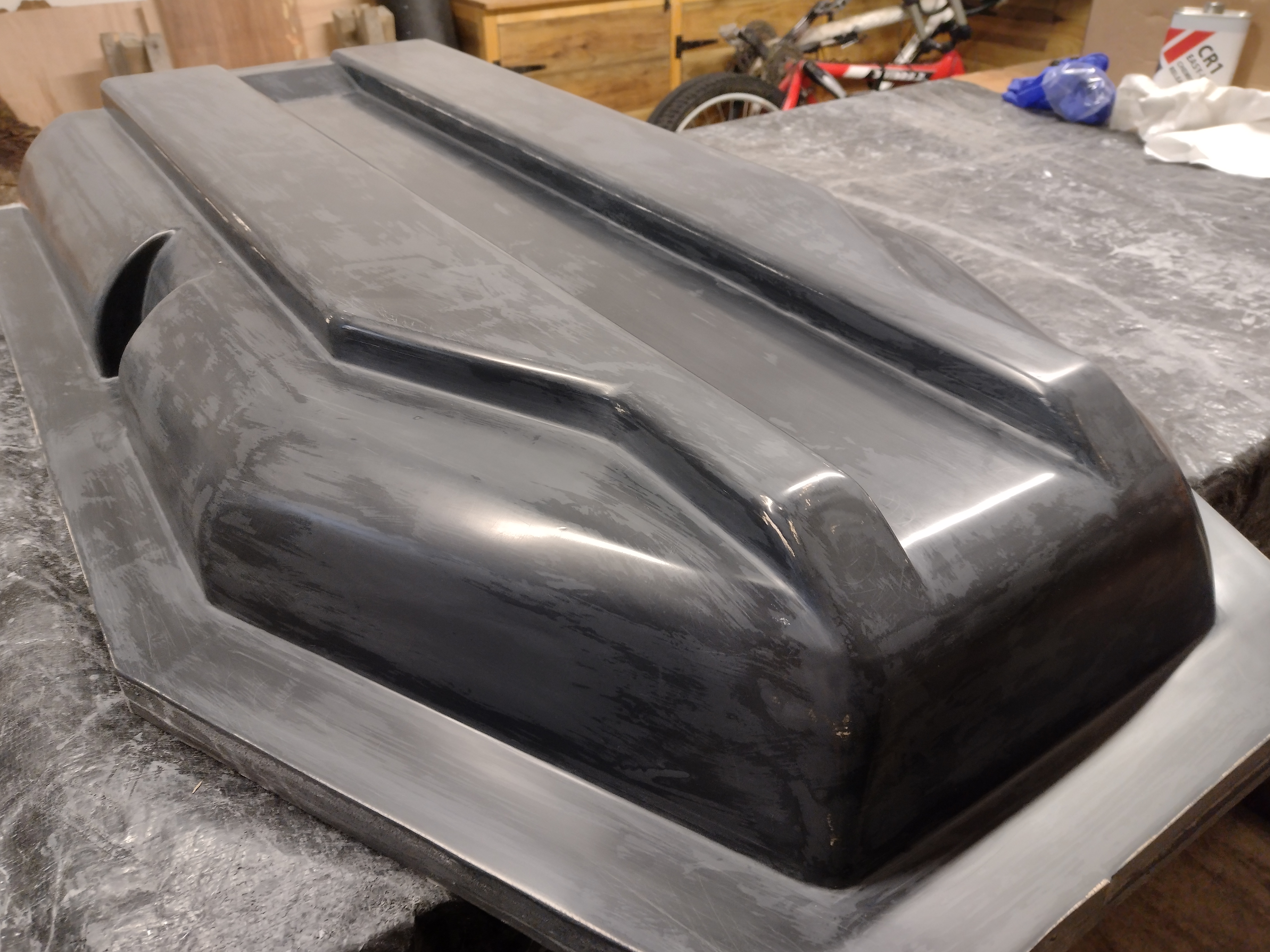
Building a glass fibre female mould

The mould, if built correctly, should allow us to make almost unlimited copies of the stretcher tray. It needs to be robust enough to survive long periods in storage but be ready to produce new parts after little more than a quick polish. I opted to use Easy Composites’ moulding system, and I’m glad I did, as it made the moulding process relatively quick and painless. The black gelcoat is first applied to the prepared plug, followed by a layer of fine glass fibre to support it. Finally, several thick layers of glass fibre are applied to give the mould its structural strength, and prevent it bending or warping. Each of these stages is fraught with potential pitfalls, any of which could damage the plug and set me back months. In fact, this project reminded me that the whole discipline of composites manufacture is a near-constant stream of potential disasters, narrowly averted through diligent background reading, experience, intuition or luck.

Further considerations: the working area had to be at a temperature of 18-25 C, tricky to achieve in a Scottish shed in November. The smell of styrene from the polyester resin is so strong that it lingers in hair and clothes for days, even after numerous washes. Every chemical component is in some way bad for you, which is unfortunate as you end up plastered in the stuff despite your best efforts at PPE. Once mixed, the resin gives you a working time of about 15 minutes before it starts to cure, which is unfortunate if you’ve embarked on a 40 minute project. If there’s more than a little resin left in the pot it will exotherm violently, smoking or even igniting to let you know you’ve left it too long!

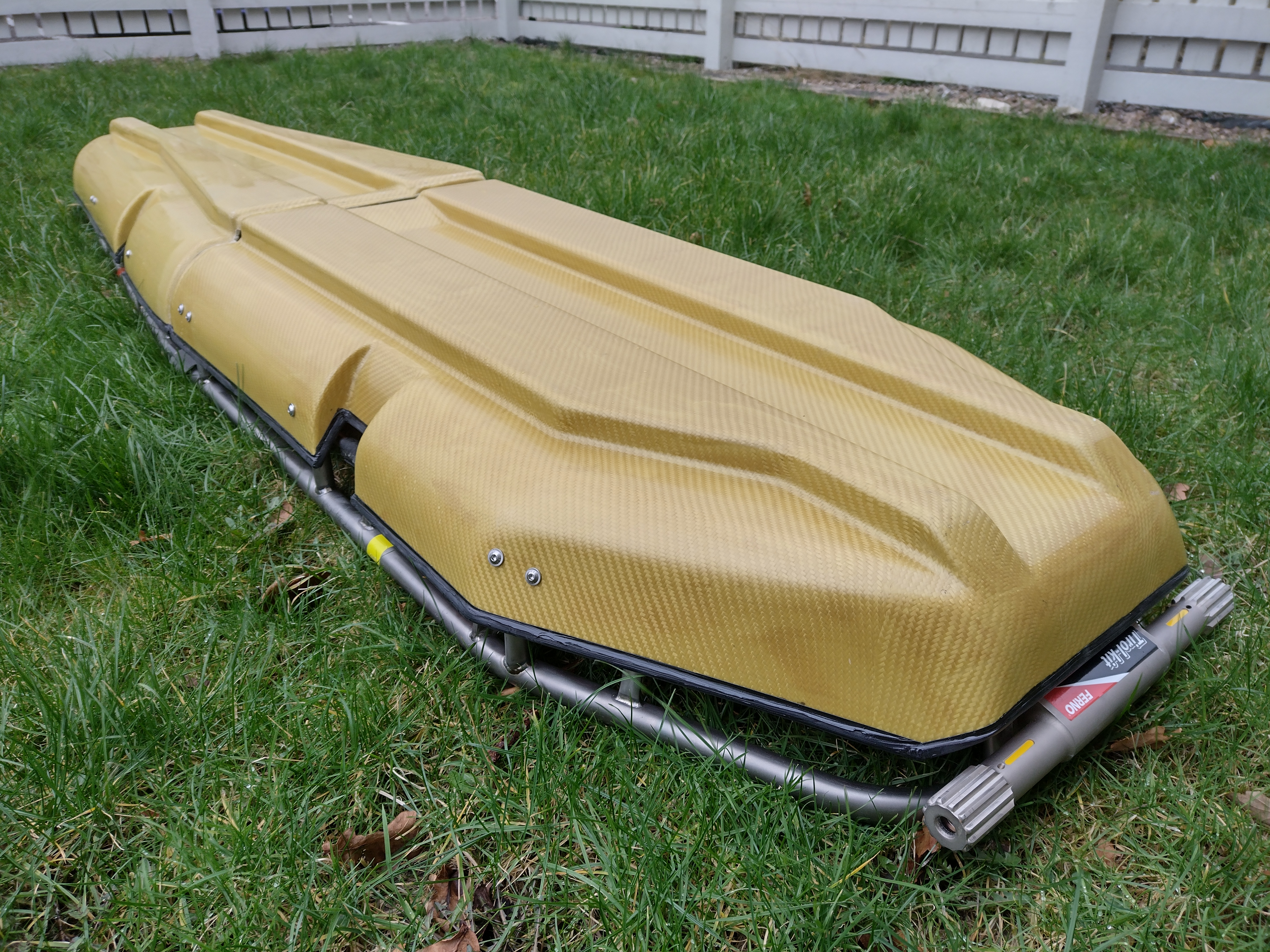
Building a Kevlar tray for field testing

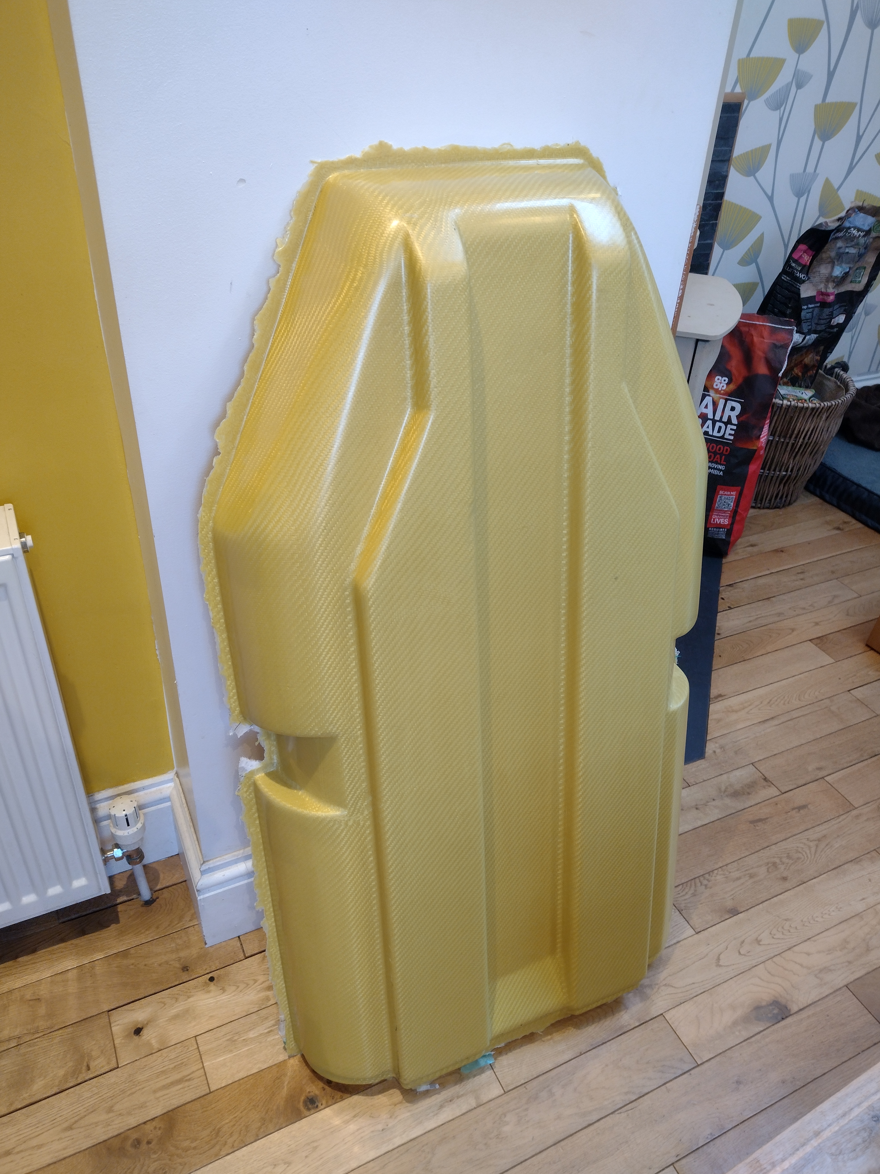
The only way to find out whether the moulded shape would be suitable for ‘real world’ conditions is to make a part and see how it performs in typical rescue scenarios. I chose to make the part from Kevlar which is a high-end composite reinforcement fabric, known mainly for its incredible toughness. It is also stronger and lighter than most other common reinforcements with the exception of carbon fibre, but carbon is very brittle so is not suitable for rough handling.

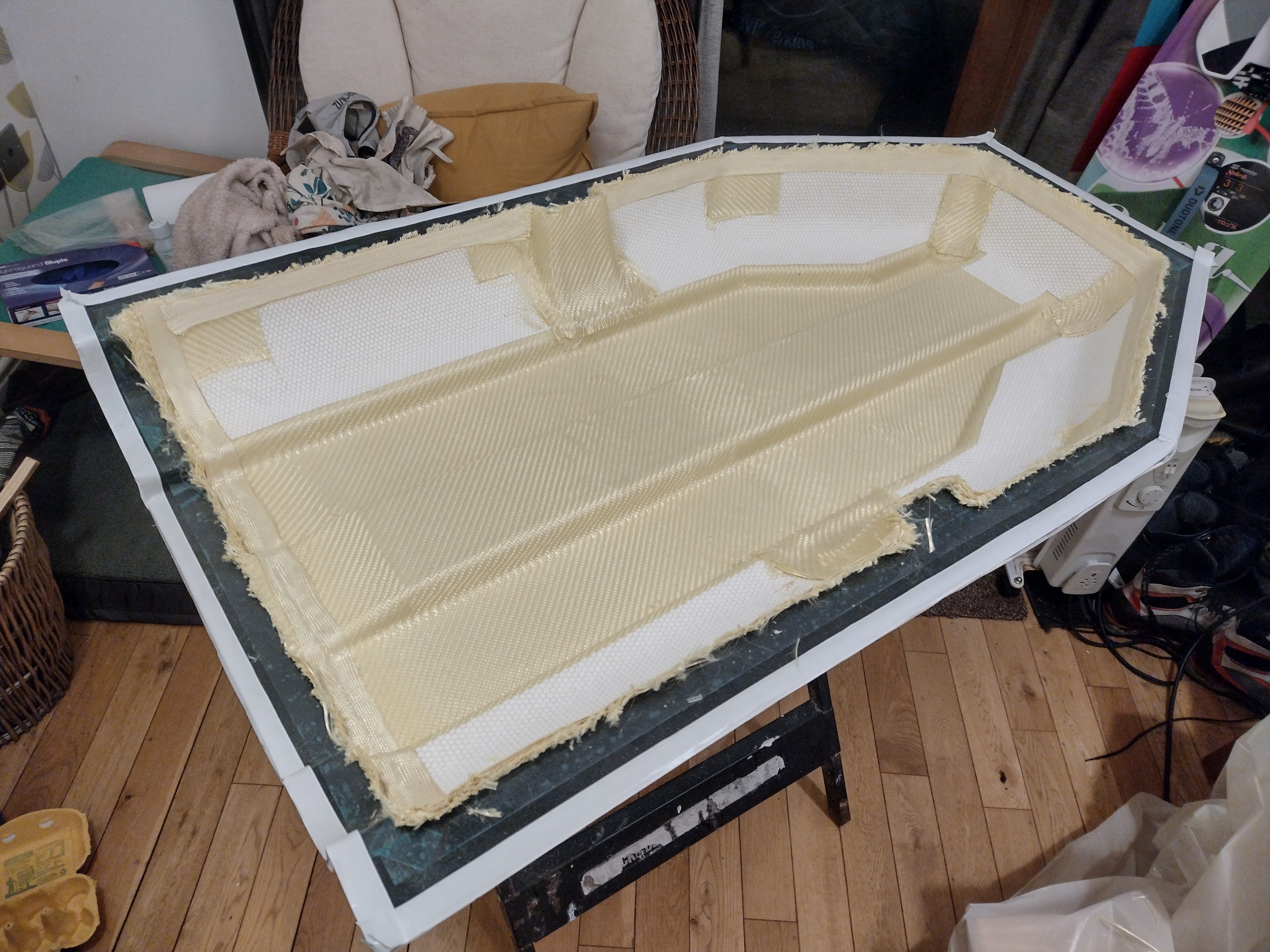
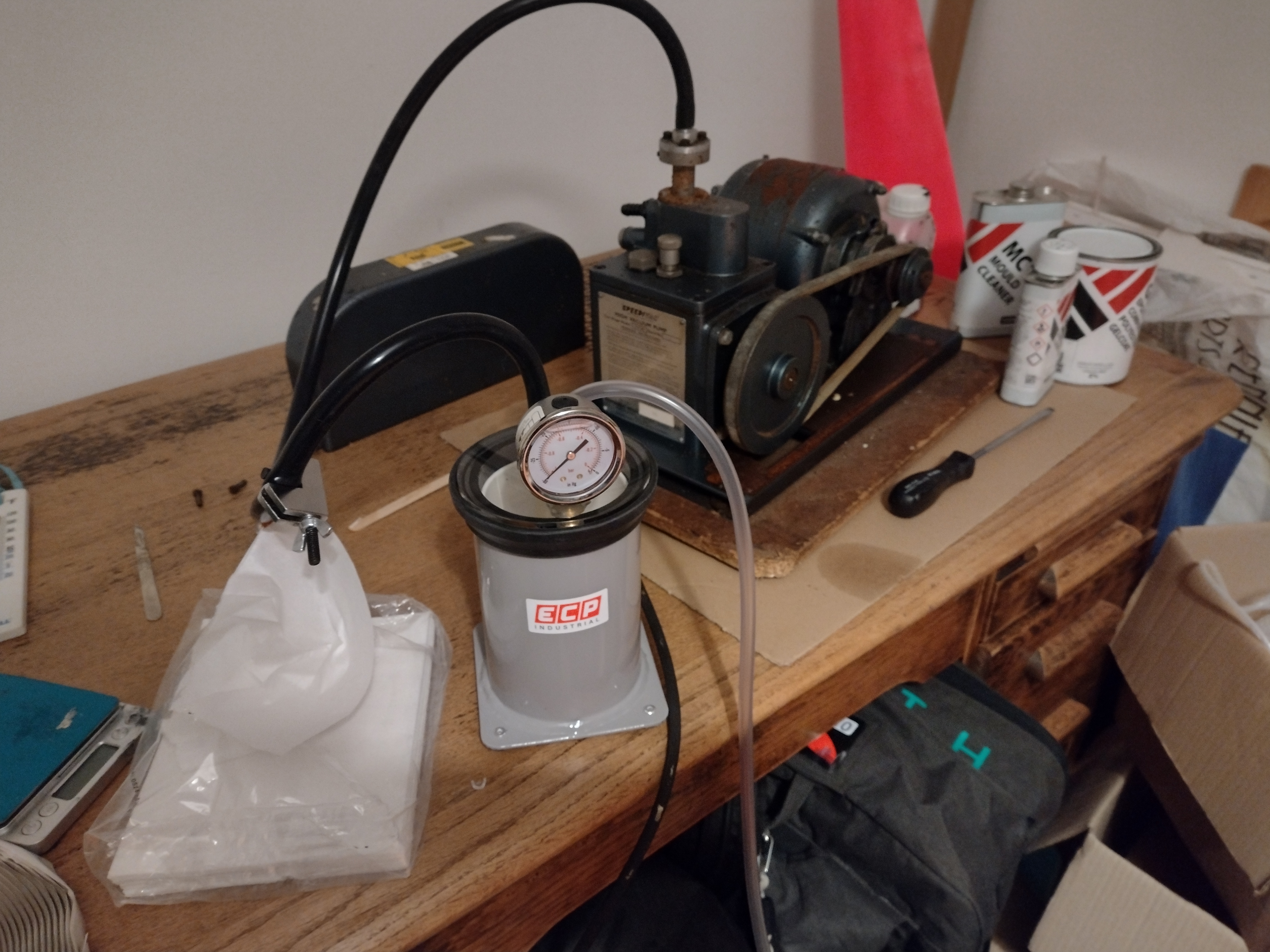
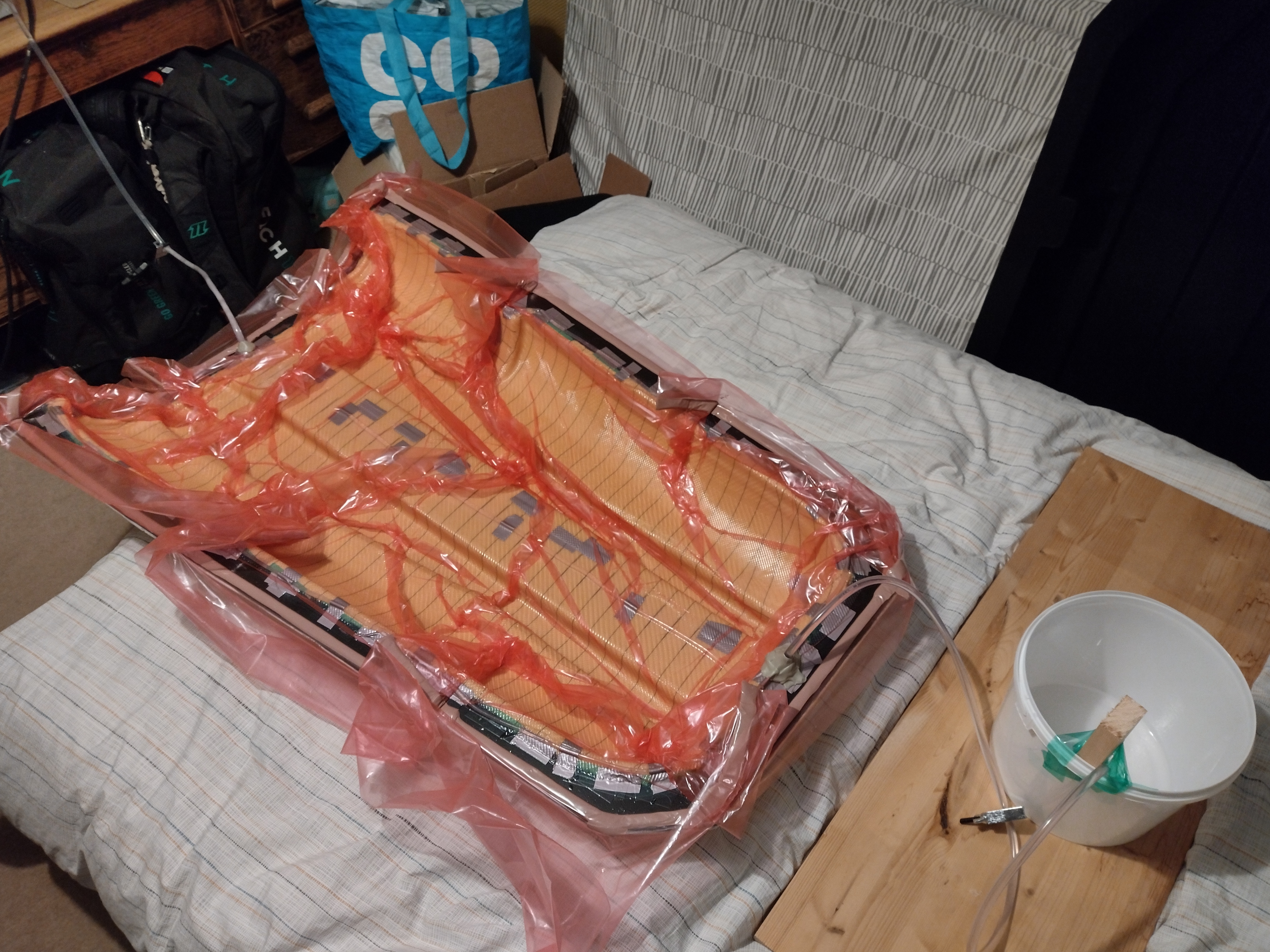
I chose to use a technique known as resin infusion. This involves laying the dry fibre layers into the mould, aided by light use of spray glue. The whole structure is put in a sealed bag and a vacuum drawn. Epoxy resin is then allowed to ‘infuse’ through the part, drawn through the dry fabric by the vacuum. If all goes to plan you are left with the perfect composite structure: just the right proportion of resin with no air bubbles. I designed the fabric layup to prioritise stiffness at the lowest weight. Extra layers were added in high impact and wear areas.

There are literally books written on the resin infusion technique, and I’ve had some experience of it previously, but let’s just say that it takes no prisoners. Even the tiniest leak in the seal of the vacuum, a poor decision in the flow channels to allow resin to spread, a pump failure, a forced error under time pressure… all spell disaster! By the skin of my teeth I got away with it and produced the two Kevlar halves. Both released from the mould with minimum fuss, leaving great-looking parts.

Finishing up

The only thing remaining was to trim the Kevlar tray parts down to size, tidy them up and fit them to the stretcher. Trimming a material that’s designed primarily for resistance to abrasion is a substantial task in itself, as my various blunted grinder blades can attest. However, it bodes well for its longevity when it’s being dragged over rocks in the field.

The completed stretcher, ready to go

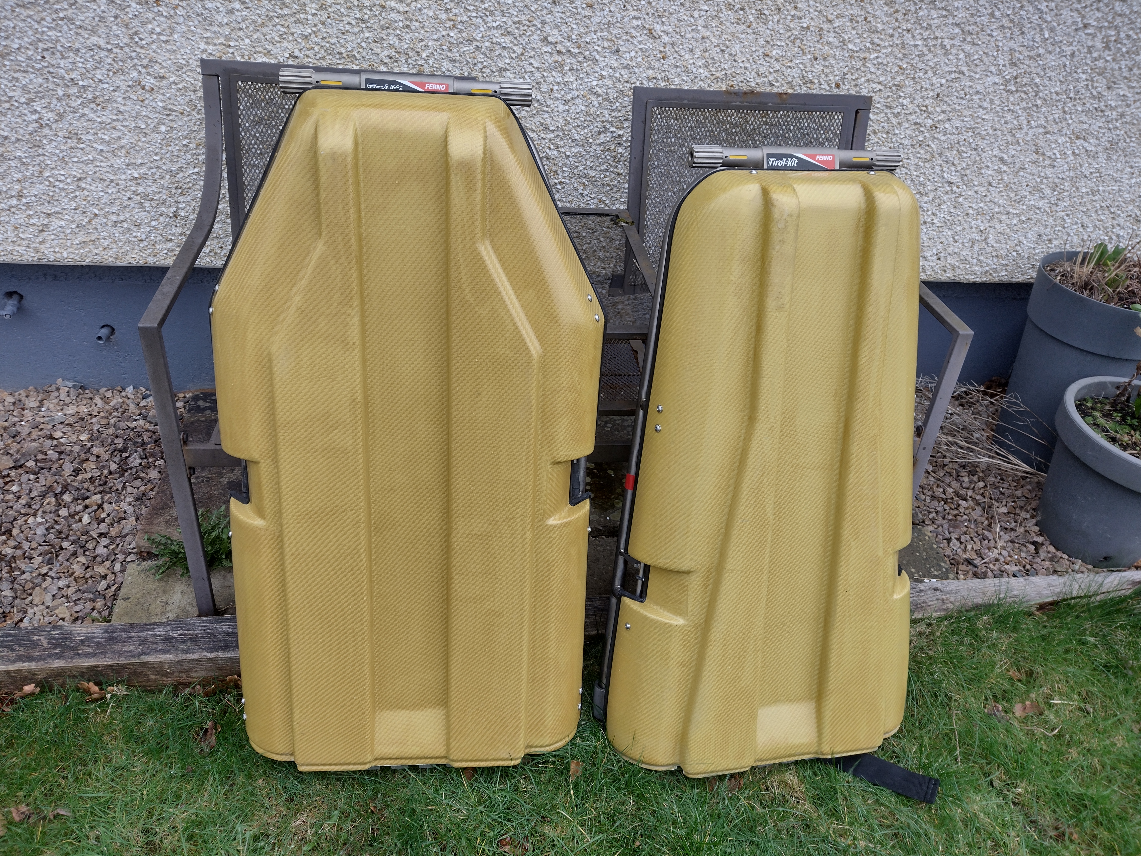
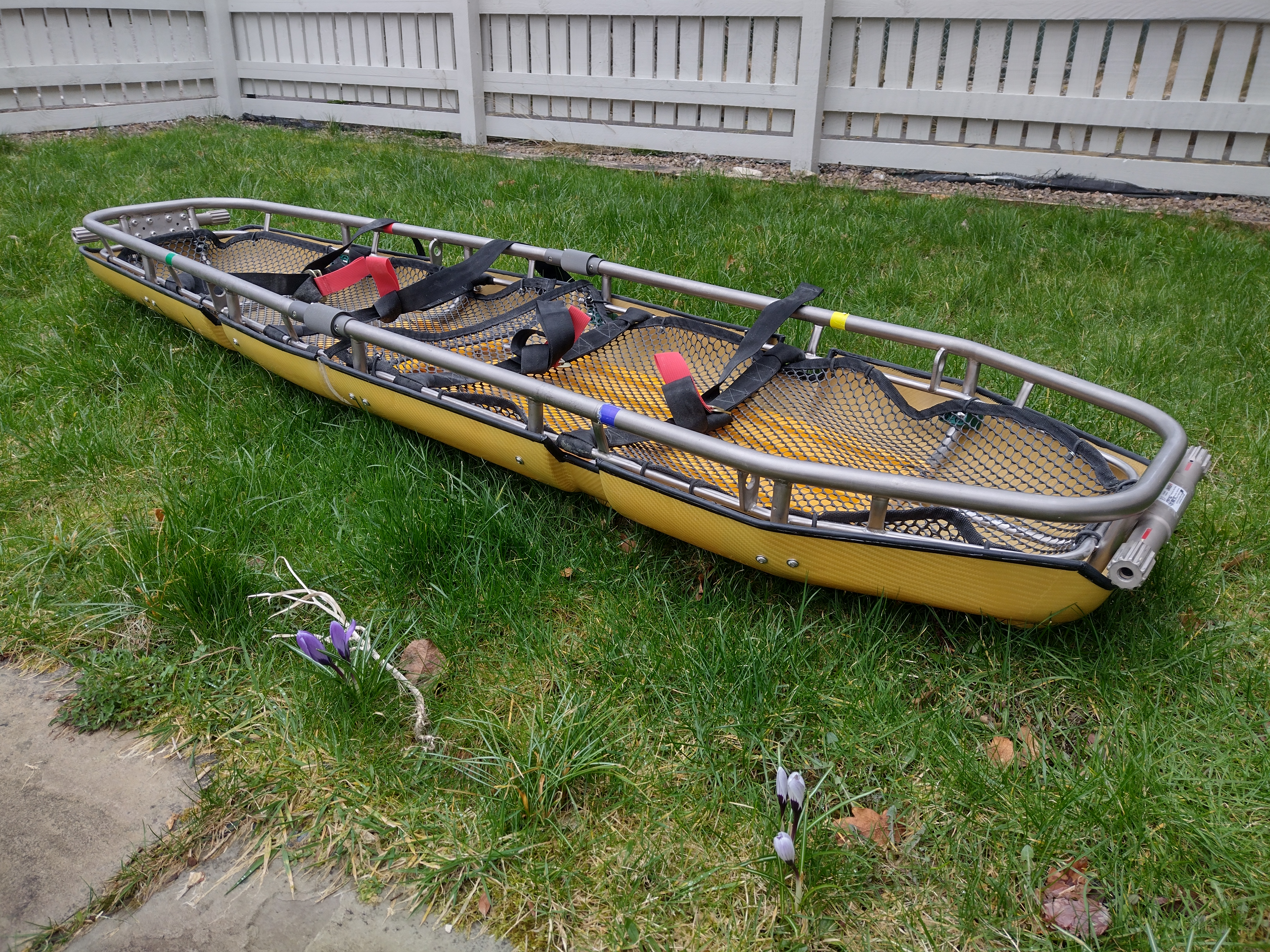
I’ve now handed the completed stretcher back to Glencoe Mountain Rescue, and hopefully it will pave the way for a replacement for the time-served MacInnes design.

New paper published: “Exceptional atmospheric conditions in June 2023 generated a northwest European marine heatwave which contributed to breaking land temperature records”

This paper was led by the UK Met Office and breaks down the nature, causes and future likelihood of the extreme marine heatwave to impact UK shelf waters in June 2023. I contributed robotic glider observations illustrating the onset and deepening of the warm surface waters west of the UK.

Glider and mooring observations during the June 2023 marine heatwave

Abstract: The Northwest European shelf experienced unprecedented surface temperature anomalies in June 2023 (anomalies up to 5 °C locally, north of Ireland). Here, we show the shelf average underwent its longest recorded category II marine heatwave (16 days). With state-of-the-art observation and modelling capabilities, we show the marine heatwave developed quickly due to strong atmospheric forcing (high level of sunshine, weak winds, tropical air) and weak wave activity under anticyclonic weather regimes. Once formed, this shallow marine heatwave fed back on the weather: over the sea it reduced cloud cover and over land it contributed to breaking June mean temperature records and to enhanced convective rainfall through stronger, warmer and moister sea breezes. This marine heatwave was intensified by the last 20-year warming trend in sea surface temperatures. Such sea surface temperatures are projected to become commonplace by the middle of the century under a high greenhouse gas emission scenario.

Berthou, S., Renshaw, R., Smyth, T., Tinker, J., Grist, J., Wihsgott, J.U., Jones, S.C., Inall, M., Nolan, G., Arnold, A., Blunn, L., Manuel, J., Gomez, B., Fraser-Leonhard, V., Hirschi, J., Lewis, H., Mahmood, S., Worsford, M., 2024. Exceptional atmospheric conditions in June 2023 generated a northwest European marine heatwave which contributed to breaking land temperature records. Nature Communications Eath & Environment, 5(1), p.287. doi: 10.1038/s43247-024-01413-8.

Slot on Channel 5 news talking about the recent marine heat wave

Following the extensive press coverage of the recent marine heatwave around UK waters, we were contacted by Channel 5 News to do a short segment on our deep water observations of the heatwave using robotic underwater gliders. Professor Stuart Cunningham described the context of the current heatwave and I talked about the role of gliders in observational oceanography.

The coverage has almost exclusively used satellite SST data as few other methods provide the real-time observations necessary for up-to-date coverage. As part of the OSNAP observation program, we maintain a robotic glider near the continental shelf edge for most of the year, so were in a prime position to observe the heatwave as it unfolded in real time.

The vertical temperature profiles provided by the glider enabled us to track the propogation of the heatwave downwards. We’ll keep tabs on how it plays out over the coming weeks.

New paper published: “Observation-based estimates of volume, heat, and freshwater exchanges between the subpolar North Atlantic interior, its boundary currents, and the atmosphere”

This is work we published in Ocean Science in early 2023. While much has been written on the transformation of water north of the OSNAP or RAPID lines, we decided to isolate and investigate the role of the subpolar gyre interior as delineated by the 1000 m isobath, using a boundary dataset comprised of Argo, CTD and EN4 reanalysis data. The circuit was closed across 47 N to the south.

Jones, S.C., Fraser, N.J., Cunningham, S.A., Fox, A.D., Inall, M.E., 2023. Observation-based estimates of volume, heat and freshwater exchanges between the subpolar North Atlantic interior, its boundary currents and the atmosphere.  Ocean Science, 19(1), pp.169–192, doi:10.5194/os-19-169-2023.

Abstract

The Atlantic Meridional Overturning Circulation (AMOC) transports heat and salt between the tropical Atlantic and Arctic Oceans. The interior of the North Atlantic Subpolar Gyre (SPG) is responsible for the much of the water mass transformation in the AMOC, and the export of this water to intensified boundary currents is crucial for projecting air-sea interaction onto the strength of the AMOC. However, the magnitude and location of exchange between the SPG and the boundary remains unclear.

Smoothed 1000 m bathymetry contour (solid black line), closed by transect across 47° N. Key locations around contour are labelled; these are used throughout this study. Dashed black line shows OSNAP line. RT: Rockall Trough, WTR: Wyville Thomson Ridge. Mean magnitude and direction of surface currents (2000-2020) derived from AVISO data shown by coloured contours and quiver arrows. Isobaths overlaid at 1000 m increments. Bathymetry contours from GEBCO bathymetry (http://www.gebco.net/).  GEBCO = General Bathymetry Chart of the Oceans.

We present a novel climatology of the SPG boundary using quality controlled CTD and Argo hydrography, defining the SPG interior as the oceanic region bounded by 47° N and the 1000m isobath.

Gridded boundary product plotted by distance along the 1000 m contour travelling anti-clockwise around the basin.  Annual means shown.  (a) conservative temperature (̊C), (b) absolute salinity (g kg-1), (c) density (σ0, kgm-3), (d) geostrophic velocities across the boundary perpendicular to the 1000 m depth contour (cm s-1, positive into the interior, negative out of the interior, colour map intervals of 0.25 cm s-1 with selected contours shown).  Density contours relevant to overturning processes (Fig. 9) shown by black dashed lines in (c) and (d).  The transition to the 47° N section, and from gridded CTD to EN4 climatology data, is delineated by the dashed white line. Key locations around boundary labelled. FSC: Faroe-Shetland Channel, southernmost point of Iceland, RR: Reykjanes Ridge (southern tip), Cape Farewell, LS: Labrador Sea, Gulf Stream.

From this hydrography we find geostrophic flow out of the SPG around much of the boundary with minimal seasonality. The horizontal density gradient is reversed around West Greenland, where the geostrophic flow is into the SPG.

Geostrophic transport perpendicular to contour, into the SPG positive. a) Depth integrated volume transport between 0 and 1000 m for each grid cell (timeseries/annual mean).  Quiver arrows show magnitude of transport across grid cell, and are constrained to be perpendicular to the section. Horizontal bins are 150 km apart around the 1000 m contour, and 1° across 47° N.  Bathymetry contours from GEBCO bathymetry (http://www.gebco.net/).  GEBCO = General Bathymetry Chart of the Oceans. (b) Cumulative volume transport around basin, for each season. Key locations around boundary labelled as for Fig. 3, vertical dashed lines denote OSNAP crossings.

Surface Ekman forcing drives net flow out of the SPG in all seasons with pronounced seasonality, varying between 2.45 ± 0.73 Sv in the summer and 7.70 ± 2.90 Sv in the winter. We estimate heat advected into the SPG to be between 0.14 ± 0.05 PW in the winter and 0.23 ± 0.05 PW in the spring, and freshwater advected out of the SPG to be between 0.07 ± 0.02 Sv in the summer and 0.15 ± 0.02 Sv in the autumn. These estimates approximately balance the surface heat and freshwater fluxes over the SPG domain. Overturning in the SPG varies seasonally, with a minimum of 6.20 ± 1.40 Sv in the autumn and a maximum of 10.17 ± 1.91 Sv in the spring, with surface Ekman the most likely mediator of this variability.

(a) Overturning stream function ψ for full SPG boundary in density space between surface and seabed using corrected velocities for sub-1000 m currents.  Density of maximum overturning, and that of secondary peak where applicable, highlighted by circles.  Densities of mean inflection points marked by horizontal grey dashed lines; these are overlaid on Fig. 3c and d.  The hatched area denotes the approximate density space impacted by the sub-1000 m correction velocities. (b) same, but for boundary contour (0-9500 km) only, (c) same, but for 47° N transect (9500 – 12700 km) only.

The density of maximum overturning is at 27.30 kgm-3, with a second, smaller maximum at 27.54 kgm-3. Upper waters (σ0 < 27.30 kgm-3) are transformed in the interior then exported as either intermediate water (27.30-27.54 kgm-3) in the North Atlantic Current (NAC) or as dense water (σ0 > 27.54 kgm-3) exiting to the south. Our results support the present consensus that the formation and pre-conditioning of subpolar Mode Water in the north-eastern Atlantic is a key determinant of AMOC strength.

Schematic of SPG boundary and interior processes contributing to transport through the SPG, viewed from 47° N section. The shaded rectangles on either side of the basin represent the regions in which CTD data were gathered. SC: Slope current, Net flow across 47 N above 1000 m is northward (into the SPG) and below 1000 m it is southward (out of the SPG). A net downwelling (F) is required to balance the transports in and out of the SPG.

Climate science showcase at Dynamic Earth (COP26)

A few weeks late but I thought I should add some photos of the event we attended as part of the COP26 activities. We had a great day chatting with the public about our work and demonstrating some of the robots and instruments used for physical oceanography. Dynamic Earth reported 1400 visitors throughout the day, one of their busiest public engagement events ever! Great to see so many folk after so much isolation over the past year.

Great that the seaglider model I built years ago has been such a valuable outreach tool. It’s still going strong, albeit with a few knocks and scratches. It looks more like the real thing as a result! More information on its construction here: https://samcjones.com/science-media/seaglider-model/

DY120 cruise animation

Following on from our recent successful completion of the OSNAP cruise on board RRS Discovery, I made a little animation showing how the objectives of the cruise were completed, and how compliant the weather was throughout. The North Atlantic, not known for respecting cruise schedules during the autumn and winter, allowed us a window just long enough to complete all the mooring turnarounds, CTDs and Argo deployments. Of note is the 3-day run back from IB3 in the Iceland Basin to complete the final mooring and get behind the Hebrides before the next low-pressure system arrived. The following Wednesday, waves up to 29 m were recorded west of Ireland, more or less where we’d been the previous week! Along with getting out during COVID, this seems like another aspect of DY120 worth celebrating.

Also on the animation is SAMS glider “Bowmore”, which was deployed in September and will run transects of the shelf edge current throughout the winter. A classic ‘tortoise and hare’ scenario: she doesn’t get anywhere fast, but who’s still out there gathering data long after we’ve run for shelter!

The history of AMOC study, blog post written during the DY120 cruise

Sam Jones 16/10/20

The world’s oceans are in constant circulation. Like a vast, stately conveyer belt, water flows from the tropics to polar regions where it cools and becomes denser, pouring back along the basins and valleys of the seabed towards the lower latitudes. This flow encompasses every ocean basin and takes many hundreds of years to complete a full circuit. A striking example of this process in action is the ocean’s delayed response to climate change: since the industrial revolution, the Polar seas have been taking in additional heat and pollutants from human activities and diligently sequestering them in the deep oceans of the world, where they will reside for many years before eventually resurfacing. Not gone forever, just filed under ‘to deal with later’.
The Atlantic segment of this flow is known as the AMOC: the Atlantic Meridional Overturning Circulation. ‘Meridional’ refers to the south-north nature of the flow, and ‘overturning’ describes its upwelling and downwelling components in the tropics and the poles, respectively. Despite its stately progress, the energy moved by the AMOC is staggering: roughly 1.25 Peta (1015) Watts of heat is continuously transported from the tropics towards the Atlantic Arctic via this mechanism, more than 60 times the present world energy consumption.

Schematic map of the AMOC, with RAPID and OSNAP array locations overlaid.

The idea that human activity could disrupt this immense current system was first considered in response to an unexpected result: in 1957 an ambitious hydrographic survey aimed to measure the total amount of water and heat transported by the AMOC using a line of observations between the eastern and western sides of the Atlantic ocean. This effort successfully delivered a figure for the strength of the AMOC, and a follow-up experiment in 1981 was conducted to see whether anything had changed during the 24-year interval. Contrary to expectations, the transport was found to have decreased significantly. The discrepancy was tentative evidence that this seemingly inexorable current system was slowing down.
A possible culprit for the slowdown was forthcoming: The Polar ice caps store vast amounts of fresh water, and human-induced climate change has added to existing ice melt, causing more fresh water to flow into the Polar oceans. Fresh water reduces the density of seawater so has the potential to disrupt the engine that drives the AMOC; water in the Arctic may no longer have sufficient density to sink and flow towards the tropics. This phenomenon would not be unprecedented: there is much evidence that such slowdowns occurred due to melting at the end of the last ice age, as recently as 8,200 years ago. This is the scenario portrayed in the movie ‘Day after Tomorrow’: it’s true that the warm, salty North Atlantic Current keeps Western Europe relatively mild and that a reduction in this current could lead to cooling in the northern hemisphere. That the current could ‘switch off’ in a matter of days, leading to polar super-hurricanes and an influx of wolves into New York is less scientifically rigorous, but in the interests of dramatic cinema we’ll let that slide.

After the discovery of an apparent slowdown in the AMOC, it was imperative that we learned more about the Atlantic portion of the ocean conveyer belt. How quickly was it slowing down? What would be the implications for climate in the northern hemisphere? How sensitive would it be to future changes in climate? To answer these questions, the RAPID mooring array was instigated in 2004. It comprised a line of deep ocean moorings maintained between Morocco and Florida to continuously measure the AMOC in a more comprehensive manner than had previously been possible. The data provided by this array demonstrated that the slowdown was real, but more gradual than had initially been feared. However, the scale of year-to-year and even seasonal variability in current strength was far greater than expected.

Scientists collect water samples during DY120 (Sam Jones/SAMS).

A large unknown remained: how much of the water which passes through the RAPID array reaches the Arctic to cool and sink, and how much just recirculates in the North Atlantic? To answer this question and better understand the engine which drives the AMOC, it was decided that a second array of instruments – a ‘gateway’ across the entrance to the Polar seas – was needed. This mooring array stretched from Western Scotland, via Greenland, to the east coast of Canada and was named OSNAP (the Overturning in the Sub-Polar North Atlantic Program). This international effort has been maintained since 2014 and has offered further insight into the inner workings of the ocean conveyer belt. We now know, for example, that most of the cooling and sinking occurs east of Greenland, and not in the Labrador Sea as was previously thought. In addition, most of the strong year-to-year changes in AMOC strength originate in the stormy seas of the Eastern North Atlantic where we currently find ourselves.
The moorings we are recovering during DY120 have survived for two years in the Atlantic Ocean, weathering some of the roughest seas on the planet. The data contained in these moorings adds to four years of existing OSNAP data, so increases the total duration of our time series by 50 %, a significant boost to our understanding. Each mooring consists of tens of instruments distributed along a wire, which is anchored to the seabed and kept vertical by a series of buoyant floats. Due to the depth of the ocean basins, most of the moorings are several kilometres long, so the task of recovering each mooring intact onto a relatively small vessel, downloading data and redeploying in precisely the same location is non-trivial. We have now moved from the Rockall Trough into the Iceland Basin, and each successful mooring turnaround feels like a significant triumph given the challenges in getting to this point.

Mooring recovery during DY120 (Sam Jones/SAMS).

New ICES ocean climate and atmosphere report published

The ICES Working Group on Ocean ​​Hydrography (WGOH), of which I am a chair-invited member, has just published its annual report on North Atlantic ocean conditions in 2018.  The report comprises several dozen multi-year time series of ocean observations around the North Atlantic Basin, which together paint a coherent picture of the current status of the ocean climate:  https://www.ices.dk/news-and-events/news-archive/news/Pages/Ocean-climate-2019.aspx

IMG_4344

North Atlantic ocean conditions 2018

In 2016, freshening of the upper ocean (0–1000m depth) was observed in the eastern subpolar North Atlantic. This decrease in salinity has since expanded northwards into the Nordic seas, influencing the Greenland Sea and northern Norwegian Sea to Fram Strait, as well as the southern reaches of the Barents Sea. Freshening is also observed spreading westward into the Irminger Sea and eastward into the North Sea.

Throughout the subpolar region, freshening is accompanied by moderate cooling at just a few sites, indicating that the large changes in salinity are dissociated from changes in temperature.

Freshening of central waters in the northeast Subtropical Gyre and intergyre region (Bay of Biscay, West Iberia, Gulf of Cadiz, and Canaries) was enhanced and extended deeper into the water column. In contrast to northern regions, temperatures here decreased in concert with freshening, thereby conserving water mass properties.

Coupled with atmospheric conditions, sea surface temperatures (SST) exhibited a tri-pole pattern, with warm conditions in both the subtropical and Nordic seas regions and cooler conditions in the subpolar region. A cold anomaly observed in the surface and upper ocean of the central subpolar North Atlantic intensified and expanded after weakening in 2017.

The Scotian and Northeast US shelves were warmer than normal, accompanied by notable freshening at several sites.

Extremely warm temperatures were observed near the surface in spring–summer across the Baltic Sea and the North Sea (> 1.5˚C than normal), with less pronounced warming observed from Biscay to Ireland (0.5–+1.0 ˚C).